Third Approach:Depth Based Seeding

The central idea of this approach is to take advantage of the raw depth data and the normal map of the scene to get an initial estimate of the of the object to be extracted. Then we take this estimate as basis to build the Foreground and Background Color Models, and finally we apply GrabCut on an energy function that take into account both depth and color information.

The initial estimate of the object is done using the following two criteria :

• Central and Closest is Foreground.
• External and Planar is Background

Central and Closest is Foreground

1. A random sample of pixels is taken from the central rectangle (i.e, the rectangle with sides 1/2 and in the middle of the ROI). Using K-means we identify n clusters of depth data.

2. The clusters are sorted by depth distance from closest to farthest. The closest cluster is fixed as FG. Define d₁₂,d₂₃,...,d_n-1n  the distance between consecutives cluster:.
   
   

   • If d₁₂<d_tol  the second cluster is added as FG. Otherwise it is rejected and the unique cluster associated FG is the closest one.
   • If d₂₃<m_tol d₁₂ the third cluster is added as FG. Otherwise it is rejected, and the clusters associated FG are the previous one.
   • ....
   • If d_n-1n<m_tol d_n-2n-1 the nth cluster is added as FG. Otherwise it is rejected, and the clusters associated FG are the previous one.
3. From all the pixels belonging to the clusters marked as FG we took the lowest value of depth  (minDepthFG) and the largest value of depth (maxDepthFG).

External and Planar is Background

1. The normal at each pixel of the image is calculated from the raw depth data.
2. Take a random sample of pixels in the outer annulus of  the ROI and store them in a queue.
3. Fix a normal tolerance parameter (e_n) and color tolerance parameter (e_c).
4. Pick the first pixel of the queue (p) and identify the connected set of pixels around p that satistifies the conditions, ||n_p-n_x||<e_n and ||c_p-c_x||<e_c. Call this set of pixels PN(p), and label all these pixels as belongComponent.
5. In order to confirm PN(p) as a valid plane the following two conditions must hold: 

• PN(p) is greater than 5% of image size.
•  At most 25% of PN(p) belong to the central rectangle.

If the previous conditions holds, we label all the pixels in PN(p) as planarPixels. Otherwise, we undo the belongComponent labelling, and we start to construct a new component from the next non planarPixel in the queue.

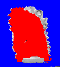
Seeding

In order to identify as BG pixels those that have a relative large depth value, belong to a planar patch, or are located near  the frontier of the rectangular selection, lets define the following  functions W_BG and W_FG that will be constructed in three steps:

First Step

 Let d_p be the depth associated to pixel p:

1. if  minDepthFG<d_p<maxDepthFG, set  W_BG(p)=1400.
2. if  d_p<minDepthFG,  set  W_BG(p)=max(1400+300(d-minDepthFG)/(maxDepthFG-minDepthFG) , 0).
3. if  d_p>maxDepthFG,  set  W_BG(p)=max(1400-300(d-maxDepthFG)/(maxDepthFG-minDepthFG) , 0). 
4. if d_p=0 (noisy depth value), set W_BG(p)=900.
5. For all p set W_FG(p)=1200.
   

Second Step

Let (i,j) be the image coordinates of pixel p ( i=1,...,r and  j=1...c )

1. Set d_center(p)=max(abs(i-(r/2))/(r/2),abs(j-(c/2))/(c/2)).
2. Set W_FG(p)=W_FG(p)+40*d_center(p).
3. Set WB_G(p)=W_BG(p)+40*(1-d_center(p)).

Third Step

1. If pixel p is planar set W_FG(p)=W_FG(p)+1200.

Once W_BG and W_FG are constructed we define the seeds as follows:

• If W_BG(p)-W_FG(p)>160, then p is a FG seed.
• If W_FG(p)-W_BG(p)>450, then p is a BG seed.

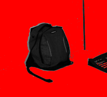
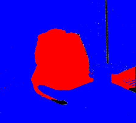
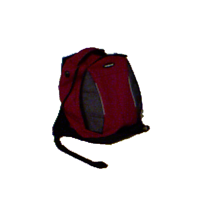
Final Results

Remarks

Pros:

• Good seeding: Using depth data in a structerd way and following certain general and reasonable criteria makes the seeding robust.
• Satisfactory results in object-background adjacency and non adjacency.

Cons:

• Parameter adjusts are required to deal with specific cases.